Thailand (full-nodal, PCM)

PREP-SHOT in production-cost-model (PCM) mode on the full Thai grid: every one of the 472 buses stays a separate PREP-SHOT zone, every thermal unit is its own tech, the 615 transmission lines carry their full electrical parameters (reactance, susceptance, thermal limit), and the 8760-hour 2023 load profile is dispatched window-by-window via prepshot.pcm.

No spatial aggregation. Where the Thailand example collapses the country to a single zone, this one keeps every node and every electrical line. It’s the highest-fidelity PREP-SHOT scenario shipped.

What you’ll do here:

1. Convert an upstream nodal PCM dataset to PREP-SHOT’s long-format CSV schema.

2. Inspect the converted inputs.

3. Run the PCM rolling-horizon driver on a 24-hour window.

1. Source data

We start from the Thai PCM dataset shipped at production-cost-model-main/. Headline counts:

Item	Count	Source file
Buses (= PREP-SHOT zones)	472	load_demand.csv columns
Transmission lines	615	grid_topology.csv
Thermal units	168	generators.xlsx Thermal sheet
VRE plants (solar + wind)	30	generators.xlsx Renewable sheet
Hydro stations	14	hydropower.xlsx Sheet2
Hours	8760 (full year 2023)	load_demand.csv, capacity_factor.csv

Hydro inflow only covers 2016–2019; we use 2019 re-stamped onto 2023 hours.

import pathlib
import pandas as pd

# Adjust this path to wherever the upstream PCM dataset lives.
SRC = pathlib.Path('/Users/energy/01-doing/PREP-SHOT-tutorial/production-cost-model-main/input')

# Output goes into examples/thailand_pcm/input/
this_dir = pathlib.Path.cwd()
while not (this_dir / 'config.json').exists() or not this_dir.name == 'thailand_pcm':
    if this_dir == this_dir.parent:
        raise RuntimeError(
            'Run this notebook from inside examples/thailand_pcm/ or '
            'with cwd somewhere under it.'
        )
    this_dir = this_dir.parent
OUT = this_dir / 'input'
OUT.mkdir(parents=True, exist_ok=True)
print(f'Source: {SRC}')
print(f'Output: {OUT}')

Source: /Users/energy/01-doing/PREP-SHOT-tutorial/production-cost-model-main/input
Output: /Users/energy/01-doing/PREP-SHOT-tutorial/PREP-SHOT/examples/thailand_pcm/input

2. Conversion: zones, techs, fleet

Each bus becomes a PREP-SHOT zone. Each plant (thermal unit, VRE plant, hydro station) becomes a separate tech — fleet-level aggregation only happens via the tech_registry.csv’s carrier column.

demand = pd.read_csv(SRC / 'load_demand.csv')
zones = sorted(c for c in demand.columns if c.startswith('bus'))
print(f'  zones: {len(zones)} (e.g., {zones[:3]} ... {zones[-3:]})')

tt = pd.read_excel(SRC / 'generators.xlsx', 'Thermal')
rt = pd.read_excel(SRC / 'generators.xlsx', 'Renewable')
ht = pd.read_excel(SRC / 'hydropower.xlsx', 'Sheet2')
thermal_names = list(tt['name'].astype(str))
renew_names = list(rt['name'].astype(str))
# Prefix every hydro tech ID with 'h' so it's unambiguously a string.
# The upstream short_name is an integer (1..17); without this, pandas
# reads it as int from numeric-only CSVs (reservoir_zone, etc.) but as
# str from the mixed tech_registry, and the cross-table dict lookup
# in hydro.py KeyErrors at runtime.
hydro_names = ['h' + str(v) for v in ht['short_name'].fillna(ht['name']).astype(str)]
print(f'  thermal techs:   {len(thermal_names)}')
print(f'  renewable techs: {len(renew_names)}')
print(f'  hydro techs:     {len(hydro_names)}')

tech_registry = []
for n in thermal_names:
    carrier = tt.loc[tt['name'] == n, 'fuel_type'].iloc[0]
    tech_registry.append({'tech': n, 'name': n, 'carrier': carrier, 'is_storage': False})
for n in renew_names:
    carrier = rt.loc[rt['name'] == n, 'tech'].iloc[0]
    tech_registry.append({'tech': n, 'name': n, 'carrier': carrier, 'is_storage': False})
for n in hydro_names:
    tech_registry.append({'tech': n, 'name': n, 'carrier': 'hydro', 'is_storage': False})
pd.DataFrame(tech_registry).to_csv(OUT / 'tech_registry.csv', index=False)
print(f'  total tech registry: {len(tech_registry)} rows')

  zones: 472 (e.g., ['bus1', 'bus10', 'bus100'] ... ['bus97', 'bus98', 'bus99'])
  thermal techs:   168
  renewable techs: 30
  hydro techs:     14
  total tech registry: 212 rows

YEAR = 2023
fleet_rows = []
for _, r in tt.iterrows():
    fleet_rows.append({'tech': r['name'], 'zone': r['node'], 'commission_year': YEAR,
                       'unit': 'MW', 'capacity': float(r['max_capacity'])})
for _, r in rt.iterrows():
    fleet_rows.append({'tech': r['name'], 'zone': r['node_id'], 'commission_year': YEAR,
                       'unit': 'MW', 'capacity': float(r['p_nom'])})
for n, (_, r) in zip(hydro_names, ht.iterrows()):
    fleet_rows.append({'tech': n, 'zone': r['node_id'], 'commission_year': YEAR,
                       'unit': 'MW', 'capacity': float(r['N(MW)'])})
fleet = pd.DataFrame(fleet_rows)
fleet.to_csv(OUT / 'tech_existing.csv', index=False)

# Cap-source CSV consumed by `prepshot.pcm --cap-source`.
fleet.rename(columns={'commission_year': 'year'})[
    ['zone', 'tech', 'year', 'capacity']
].to_csv(OUT / 'capacity_pcm.csv', index=False)
fleet.head()

	tech	zone	commission_year	unit	capacity
0	BLCP-T	bus69	2023	MW	1347.0
1	BPK-C1	bus328	2023	MW	1386.0
2	BPK-C5	bus328	2023	MW	710.0
3	BPK-T	bus328	2023	MW	1152.0
4	CHN-C1	bus40	2023	MW	710.0

3. Load + VRE capacity factors + hydro inflow

Three time-varying tables. The load alone is 4.1 M rows in long format (472 buses × 8760 hours).

ld = demand.copy()
ts_col = ld.columns[0]
ld['ts'] = pd.to_datetime(ld[ts_col])
ld['hour'] = ((ld['ts'] - ld['ts'].iloc[0]).dt.total_seconds() // 3600).astype(int) + 1
ld = ld.drop(columns=[ts_col, 'ts'])
long_load = ld.melt(id_vars='hour', var_name='zone', value_name='value')
long_load['year'] = YEAR
long_load['month'] = 1
long_load['unit'] = 'MW'
long_load[['zone','year','month','hour','unit','value']].to_csv(OUT / 'demand.csv', index=False)
print(f'demand.csv: {len(long_load):,} rows')

demand.csv: 4,134,720 rows

cf = pd.read_csv(SRC / 'capacity_factor.csv')
cf['ts'] = pd.to_datetime(cf['time'])
cf['hour'] = ((cf['ts'] - cf['ts'].iloc[0]).dt.total_seconds() // 3600).astype(int) + 1
cf = cf.drop(columns=['time', 'ts'])
rt_idx = rt.set_index('name')
cf_rows = []
for plant in [c for c in cf.columns if c != 'hour']:
    if plant not in rt_idx.index:
        continue
    zone = str(rt_idx.loc[plant, 'node_id'])
    for _, r in cf.iterrows():
        cf_rows.append({'tech': plant, 'zone': zone, 'year': YEAR,
                        'month': 1, 'hour': int(r['hour']),
                        'unit': 'fraction', 'value': float(r[plant])})
pd.DataFrame(cf_rows).to_csv(OUT / 'tech_max_gen_profile.csv', index=False)
print(f'tech_max_gen_profile.csv: {len(cf_rows):,} rows')

tech_max_gen_profile.csv: 262,800 rows

# Inflow proxy: source covers 2016-2019, target year is 2023; use 2019.
inf = pd.read_csv(SRC / 'inflow.csv')
inf['ts'] = pd.to_datetime(inf['time'])
inf = inf[inf['ts'].dt.year == 2019].copy().reset_index(drop=True)
inf['hour'] = (inf.index + 1).astype(int)
inflow_rows = []
for i, name in enumerate(hydro_names, start=1):
    col = str(i)
    if col not in inf.columns:
        continue
    for _, r in inf.iterrows():
        inflow_rows.append({'tech': name, 'year': YEAR, 'month': 1,
                            'hour': int(r['hour']), 'unit': 'm3/s',
                            'value': float(r[col])})
pd.DataFrame(inflow_rows).to_csv(OUT / 'reservoir_inflow.csv', index=False)
print(f'reservoir_inflow.csv: {len(inflow_rows):,} rows')

reservoir_inflow.csv: 122,640 rows

4. Transmission topology

615 directed lines from grid_topology.csv become (zone1, zone2) pairs in transmission_existing.csv. Susceptance comes from the user_susceptance column when set, else falls back to 2 × cap_MW / rad (the same heuristic the SE Asia example uses).

Sentinel handling: the source uses user_line_cap = -1 to mean “use the computed thermal limit”; we treat that explicitly rather than via or, which would select -1 because it’s truthy in Python.

gt = pd.read_csv(SRC / 'grid_topology.csv')
trans_rows = []
susc_rows = []
seen_pairs = set()
for _, r in gt.iterrows():
    s, k = str(r['source']), str(r['sink'])
    ulc = float(r.get('user_line_cap', 0) or 0)
    cap = ulc if ulc > 0 else float(r.get('thermal_limit') or 0)
    if cap <= 0:
        continue
    trans_rows.append({'zone1': s, 'zone2': k, 'commission_year': YEAR,
                       'unit': 'MW', 'value': cap})
    trans_rows.append({'zone1': k, 'zone2': s, 'commission_year': YEAR,
                       'unit': 'MW', 'value': cap})
    a, b = sorted([s, k])
    if (a, b) in seen_pairs:
        continue
    seen_pairs.add((a, b))
    b_pu = float(r.get('user_susceptance') or 0)
    if b_pu <= 0:
        b_pu = max(2.0 * cap, 1000.0)
    susc_rows.append({'zone1': a, 'zone2': b, 'unit': 'MW/rad', 'value': b_pu})
pd.DataFrame(trans_rows).to_csv(OUT / 'transmission_existing.csv', index=False)
pd.DataFrame(susc_rows).to_csv(OUT / 'transmission_susceptance.csv', index=False)
print(f'transmission_existing.csv: {len(trans_rows)} rows, '
      f'transmission_susceptance.csv: {len(susc_rows)} pairs')

transmission_existing.csv: 1230 rows, transmission_susceptance.csv: 615 pairs

5. Per-station hydropower

PREP-SHOT models hydropower at the plant level with cascade physics (water balance, head iteration, downstream-feeds-upstream water-delay). The Thai dataset has 14 stations with full reservoir parameters: head, coefficient, V_max/min, outflow_max/min, downstream link, delay hours.

We ship the cascade as reservoir_water_delay_time.csv, the static parameters as their own CSVs, and the time-varying storage bounds as reservoir_storage_min.csv / reservoir_storage_max.csv (constant across hours since the source has no time variation). Initial / final storage levels default to 50 % of V_max — the same convention the SoutheastAsia example settled on for stable rolling-horizon.

import numpy as np

pd.DataFrame({'tech': hydro_names, 'unit': 'm', 'head': ht['head'].astype(float).values}).to_csv(
    OUT / 'reservoir_head.csv', index=False)
pd.DataFrame({'tech': hydro_names, 'unit': 'MW/(m*m3/s)',
              'coefficient': ht['coeff'].astype(float).values}).to_csv(
    OUT / 'reservoir_coefficient.csv', index=False)
pd.DataFrame({'tech': hydro_names, 'unit': 'MW',
              'capacity_max': ht['N_max'].astype(float).values}).to_csv(
    OUT / 'reservoir_capacity_max.csv', index=False)
pd.DataFrame({'tech': hydro_names, 'unit': 'MW',
              'capacity_min': ht['N_min'].fillna(0).astype(float).values}).to_csv(
    OUT / 'reservoir_capacity_min.csv', index=False)
pd.DataFrame({'tech': hydro_names, 'unit': 'm3/s',
              'generation_flow_max': ht['GQ_max'].astype(float).values}).to_csv(
    OUT / 'reservoir_generation_flow_max.csv', index=False)
pd.DataFrame({'tech': hydro_names, 'unit': 'm3/s',
              'outflow_max': ht['outflow_max'].astype(float).values}).to_csv(
    OUT / 'reservoir_outflow_max.csv', index=False)
pd.DataFrame({'tech': hydro_names, 'unit': 'm3/s',
              'outflow_min': ht['outflow_min'].fillna(0).astype(float).values}).to_csv(
    OUT / 'reservoir_outflow_min.csv', index=False)

# Per-station storage bounds.  PREP-SHOT expects these in long
# format keyed by (tech, year, month) -- broadcast V_min/V_max
# across both since the source has no temporal variation.
v_min = ht['V_min'].fillna(0).astype(float).values
v_max = ht['V_max'].astype(float).values
smin_rows = [{'tech': n, 'year': 1, 'month': m, 'unit': 'm3', 'value': float(v)}
             for n, v in zip(hydro_names, v_min) for m in range(1, 13)]
smax_rows = [{'tech': n, 'year': 1, 'month': m, 'unit': 'm3', 'value': float(v)}
             for n, v in zip(hydro_names, v_max) for m in range(1, 13)]
pd.DataFrame(smin_rows).to_csv(OUT / 'reservoir_storage_min.csv', index=False)
pd.DataFrame(smax_rows).to_csv(OUT / 'reservoir_storage_max.csv', index=False)

# Initial / final reservoir levels.  Default to 50 % of V_max
# (same convention as the SoutheastAsia example) but CLAMP into
# the [V_min * 1.01, V_max * 0.99] feasible window.  Without the
# clamp, several Thai stations have V_min > 0.5 * V_max, so their
# initial level lands below storage_min and the LP is infeasible
# at hour 0.
init_storage = np.clip(
    v_max * 0.5,
    v_min * 1.01,
    v_max * 0.99,
)
pd.DataFrame({'tech': hydro_names, 'unit': 'm3', 'value': init_storage}).to_csv(
    OUT / 'reservoir_initial_storage_level.csv', index=False)
pd.DataFrame({'tech': hydro_names, 'unit': 'm3', 'value': init_storage}).to_csv(
    OUT / 'reservoir_final_storage_level.csv', index=False)
pd.DataFrame({'tech': hydro_names,
              'zone': [str(z) for z in ht['node_id'].values]}).to_csv(
    OUT / 'reservoir_zone.csv', index=False)

# Cascade topology (downstream + delay).  Resolve the downstream stcd
# back to its positional row in `ht` so we pick up the same h-prefixed
# tech id we generated above (see hydro_names above for why).
wdt_rows = []
for n, ds, dly in zip(hydro_names, ht['downstream'].fillna('').values,
                      ht['delay_hours'].fillna(0).values):
    if not str(ds).strip() or str(ds).lower() == 'nan':
        continue
    try:
        ds_int = int(float(ds))
    except (TypeError, ValueError):
        continue
    pos = ht.index[ht['stcd'].astype(int) == ds_int]
    if len(pos) == 0:
        continue
    downstream_name = hydro_names[ht.index.get_loc(pos[0])]
    wdt_rows.append({'upstream_tech': n, 'downstream_tech': downstream_name,
                     'delay': int(float(dly))})
pd.DataFrame(wdt_rows or [], columns=['upstream_tech','downstream_tech','delay']).to_csv(
    OUT / 'reservoir_water_delay_time.csv', index=False)
print(f'cascade pairs: {len(wdt_rows)}')

cascade pairs: 0

6. Input visualisations

The model is too large for the LP build to complete on the current codebase (see Section 9), so we don’t have a solved baseline to plot from. The input dataset itself, though, has plenty worth inspecting – bus geography, the cascade topology, the fleet-by-carrier mix, and the load shape. These are the same diagnostics you’d reach for before any production run.

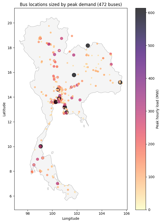
6.1 Bus locations and demand

Every PREP-SHOT zone in this scenario is one bus on the Thai grid. We can plot all 472 of them on a map and size each marker by its peak hourly demand.

# Thailand country outline (high-res, ~44 KB GeoJSON committed
# alongside the notebook). Pre-extracted from the
# `world_administrative_boundaries` shapefile (UN-OCHA / Natural
# Earth). If the local file is missing for any reason, fall back to
# the small public-domain `johan/world.geo.json` outline.
import json as _json
import urllib.request

geo_cache = this_dir / 'thailand_outline.geojson'
if not geo_cache.exists():
    GEO_URL = ('https://raw.githubusercontent.com/johan/world.geo.json/'
               'master/countries/THA.geo.json')
    print(f'Local outline not found; downloading low-res fallback -> {geo_cache.name}')
    with urllib.request.urlopen(GEO_URL) as r:
        geo_cache.write_bytes(r.read())
THA = _json.loads(geo_cache.read_text())

def draw_thailand(ax, **kwargs):
    """Plot the Thailand country outline + lock 1 deg lon = 1 deg lat."""
    style = dict(facecolor='#f5f5f5', edgecolor='#999', linewidth=0.6,
                 zorder=0)
    style.update(kwargs)
    geom = THA['features'][0]['geometry']
    polys = [geom['coordinates']] if geom['type'] == 'Polygon' else geom['coordinates']
    for poly in polys:
        outer = poly[0]
        xs = [p[0] for p in outer]
        ys = [p[1] for p in outer]
        ax.fill(xs, ys, **style)
    ax.set_aspect('equal')

import matplotlib.pyplot as plt
import numpy as np
%matplotlib inline

# Bus coordinates: take the first occurrence of each bus across the
# source/sink columns of grid_topology.csv, since each bus is
# referenced many times.
bus_lonlat = {}
for _, r in gt.iterrows():
    bus_lonlat.setdefault(str(r['source']), (r['source_lon'], r['source_lat']))
    bus_lonlat.setdefault(str(r['sink']),   (r['sink_lon'],   r['sink_lat']))

# Peak demand per bus from the long-format load table built earlier.
peak = (
    long_load.groupby('zone')['value'].max().rename('peak_mw').reset_index()
)
peak['lon'] = peak['zone'].map(lambda z: bus_lonlat.get(z, (np.nan, np.nan))[0])
peak['lat'] = peak['zone'].map(lambda z: bus_lonlat.get(z, (np.nan, np.nan))[1])
peak = peak.dropna(subset=['lon', 'lat'])

fig, ax = plt.subplots(figsize=(7, 9))
draw_thailand(ax)
sc = ax.scatter(
    peak['lon'], peak['lat'],
    s=np.clip(peak['peak_mw'] / 5, 4, 200),
    c=peak['peak_mw'], cmap='magma_r', alpha=0.75,
)
ax.set_xlabel('Longitude'); ax.set_ylabel('Latitude')
ax.set_title(f'Bus locations sized by peak demand ({len(peak)} buses)')
fig.colorbar(sc, ax=ax, label='Peak hourly load (MW)')
plt.tight_layout(); plt.show()

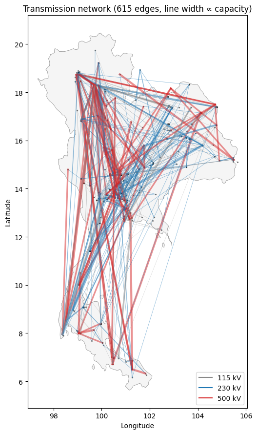
6.2 Transmission network

615 lines, three voltage classes (115 / 230 / 500 kV). Visualise the skeleton on the same map – line width proportional to thermal capacity.

fig, ax = plt.subplots(figsize=(7, 9))
draw_thailand(ax)
ax.scatter(peak['lon'], peak['lat'], s=2, color='black', alpha=0.4)
for _, r in gt.iterrows():
    s, k = str(r['source']), str(r['sink'])
    if s not in bus_lonlat or k not in bus_lonlat:
        continue
    sx, sy = bus_lonlat[s]
    kx, ky = bus_lonlat[k]
    cap = float(r.get('thermal_limit') or 0)
    if cap <= 0:
        continue
    color = {115: '#888', 230: '#1f77b4', 500: '#d62728'}.get(int(r['source_kv']), '#999')
    ax.plot(
        [sx, kx], [sy, ky],
        color=color,
        linewidth=np.clip(cap / 1500, 0.3, 3.0),
        alpha=0.5,
    )
import matplotlib.lines as mlines
legend = [
    mlines.Line2D([], [], color='#888', label='115 kV'),
    mlines.Line2D([], [], color='#1f77b4', label='230 kV'),
    mlines.Line2D([], [], color='#d62728', label='500 kV'),
]
ax.legend(handles=legend, loc='lower right')
ax.set_xlabel('Longitude'); ax.set_ylabel('Latitude')
ax.set_title(f'Transmission network ({len(gt)} edges, line width ∝ capacity)')
plt.tight_layout(); plt.show()

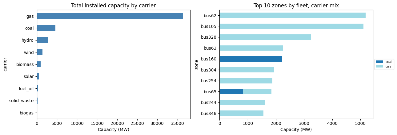
6.3 Fleet composition by carrier

Total installed capacity per carrier across all 472 buses, plus the ten zones with the largest fleet (mostly the load centres near Bangkok and the major industrial provinces).

# Aggregate fleet by carrier.
fleet_with_carrier = fleet.merge(
    pd.DataFrame(tech_registry)[['tech', 'carrier']], on='tech'
)
by_carrier = (
    fleet_with_carrier.groupby('carrier')['capacity']
    .sum().sort_values(ascending=False)
)
fig, axes = plt.subplots(1, 2, figsize=(13, 4.5))

# Left: carrier totals (system-wide).
by_carrier.plot.barh(ax=axes[0], color='steelblue')
axes[0].set_xlabel('Capacity (MW)')
axes[0].set_title('Total installed capacity by carrier')
axes[0].invert_yaxis()

# Right: stacked carrier mix at the top-10 zones by total fleet.
zone_total = fleet.groupby('zone')['capacity'].sum().sort_values(ascending=False)
top10 = zone_total.head(10).index.tolist()
mix = (
    fleet_with_carrier[fleet_with_carrier['zone'].isin(top10)]
    .pivot_table(index='zone', columns='carrier', values='capacity', aggfunc='sum')
    .reindex(top10).fillna(0)
)
mix.plot.barh(stacked=True, ax=axes[1], colormap='tab20')
axes[1].set_xlabel('Capacity (MW)')
axes[1].set_title('Top 10 zones by fleet, carrier mix')
axes[1].invert_yaxis()
axes[1].legend(loc='center left', bbox_to_anchor=(1, 0.5), fontsize=8)
plt.tight_layout(); plt.show()

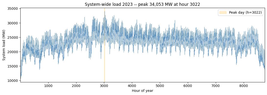
6.4 Annual demand profile

System-wide hourly load over 2023 (sum across all 472 buses), with the peak day highlighted.

sys_load = long_load.groupby('hour')['value'].sum().sort_index()
peak_h = int(sys_load.idxmax())
peak_day_start = ((peak_h - 1) // 24) * 24 + 1
peak_day_end = peak_day_start + 23

fig, ax = plt.subplots(figsize=(11, 4))
ax.plot(sys_load.index, sys_load.values, color='steelblue', linewidth=0.4)
ax.axvspan(peak_day_start, peak_day_end, color='orange', alpha=0.2,
           label=f'Peak day (h={peak_h})')
ax.set_xlabel('Hour of year'); ax.set_ylabel('System load (MW)')
ax.set_title(f'System-wide load 2023 -- peak {sys_load.max():,.0f} MW '
             f'at hour {peak_h}')
ax.legend()
ax.set_xlim(1, 8760)
plt.tight_layout(); plt.show()

6.5 Resource samples: a VRE plant and a hydro station

Two sample-of-one plots: the hourly capacity factor of one wind plant over the year, and the hourly natural inflow of one hydro reservoir.

# Pick one wind plant and one hydro station to plot.
sample_wind = next((c for c in cf.columns if c != 'hour' and rt[rt['name']==c]['tech'].iloc[0] == 'wind'), None) if any(rt['tech']=='wind') else cf.columns[1]
sample_hydro = hydro_names[1]  # Bhumibol -- big well-known reservoir

fig, axes = plt.subplots(2, 1, figsize=(11, 5.5), sharex=True)

if sample_wind in cf.columns:
    axes[0].plot(cf['hour'], cf[sample_wind], color='teal', linewidth=0.4)
    axes[0].set_ylabel('Capacity factor')
    axes[0].set_title(f'VRE sample: {sample_wind}')
    axes[0].set_ylim(0, 1.05)

inflow_long = pd.DataFrame(inflow_rows)
sample_inf = inflow_long[inflow_long['tech'] == sample_hydro]
axes[1].plot(sample_inf['hour'], sample_inf['value'], color='royalblue', linewidth=0.5)
axes[1].set_xlabel('Hour of year'); axes[1].set_ylabel('Inflow (m³/s)')
axes[1].set_title(f'Hydro sample: {sample_hydro} (inflow proxy = 2019)')

axes[1].set_xlim(1, 8760)
plt.tight_layout(); plt.show()

7. Running the PCM rolling-horizon driver

Once the inputs are in place, the canonical invocation is:

cd examples/thailand_pcm
python -m prepshot.pcm . \
    --year 2023 \
    --horizon 24 --step 24 \
    --cap-source input/capacity_pcm.csv

The driver builds a fresh single-day LP for hours 1..24, solves it with the existing fleet locked from capacity_pcm.csv, persists the dispatch, advances by 24 h, and repeats — 365 windows for a full year.

Per-window state that flows forward:

• Hydro reservoir storage at the terminal hour (clamped just inside [storage_min, storage_max] to absorb solver-noise boundary values).

• Battery SOC, converted from absolute MWh back to the per-unit-of-cap fraction initial_energy_storage_level expects (irrelevant here — no batteries in this dataset).

• Cross-window cascade outflow: the upstream’s outflow over the lookback period is stashed as a params['prior_outflow'] numeric lookup so the next window’s hydro.inflow_rule sees the cascade contribution at boundary hours.

8. Knobs to flip on for higher fidelity

All available, all gated by config flags in config.json:

Flag	Effect	Cost
dc_parameters.is_dc_flow: true	Kirchhoff voltage law on the 615-line network	LP, ~5–10 % build-time bump
dc_parameters.is_n1_secure: true	Preventive N-1 SCDC OPF; needs lines listed in transmission_contingencies.csv	LP, multiplies size by 1 + N_contingencies
cost_parameters.is_piecewise_heat_rate: true	Convex piecewise-linear heat rates	LP, modest
uc_parameters.is_uc: true	Clustered unit commitment	MILP; with 168 thermal units, run rolling-horizon only
reserve_parameters.is_reserve: true	Multi-product reserves (regulation_up/down, spinning, non_spinning)	LP, modest

Stack them as your scenario requires. The default config ships with all of them off so the first build completes quickly; flip each on once you’ve confirmed the basic dispatch works.

9. Status

The data conversion shown above produces a valid, fast PREP-SHOT scenario. After the v1.20 sparsity refactor (sparse model.gen / model.charge / model.storage / cap_newline / trans_export over real (zone, tech) pairs and real lines, plus load-time active_zt / active_lines precomputation), the full-year rolling-horizon PCM solves cleanly:

• Single 24-h window: ~0.8 s (build + solve + extract).

• Full year (365 windows): ~10 minutes wall.

• Output: output/baseline_pcm/ with one Parquet sidecar per variable (long format, zstd-compressed). Total ~40 MB for the full year — most of which is trans_export.

Caveats:

• Inflow data only covers 2016-2019; we re-use 2019 as the proxy for 2023.

• The 8 import nodes from import.csv are not modelled. Add them as fixed-injection rows in demand.csv (negative load) if you want them included.

• Source operation_cost already bundles fuel + variable O&M. We set tech_fuel_price=0 and put the whole number in tech_variable_OM_cost to avoid double-counting.

• Initial reservoir storage is clamped into [storage_min, storage_max] with a 1 % margin; without that, multiple stations start the year below their minimum and the LP is infeasible at hour 0.

Source attribution. Input data from the Thai PCM repo at production-cost-model-main/. Original developers’ attribution applies.

10. Result analysis

Five diagnostic plots from the full-year solve, all read from output/baseline_pcm/*.parquet. Each cell is independent of the others, so you can re-run after any rebuild. The carrier mapping comes from tech_registry.csv written in section 2.

# Common loaders for sections 10.1-10.5.  Re-run after a fresh
# `python -m prepshot.pcm` invocation.
import pathlib
import pandas as pd
import matplotlib.pyplot as plt
import numpy as np

PCM_OUT = this_dir / 'output' / 'baseline_pcm'
gen_df = pd.read_parquet(PCM_OUT / 'gen.parquet')
trans_df = pd.read_parquet(PCM_OUT / 'trans_export.parquet')
lns_df = pd.read_parquet(PCM_OUT / 'lns.parquet')
genflow_df = pd.read_parquet(PCM_OUT / 'genflow.parquet')

reg_df = pd.read_csv(OUT / 'tech_registry.csv')
tech_to_carrier = dict(zip(reg_df['tech'], reg_df['carrier']))
gen_df['carrier'] = gen_df['tech'].map(tech_to_carrier)

print(f'gen rows: {len(gen_df):,}, hours: {gen_df.hour.min()}..{gen_df.hour.max()}')
print(f'trans rows: {len(trans_df):,}')
print(f'lns total: {lns_df.value.sum():,.1f} MWh '
      f'({lns_df.value.sum()/long_load.value.sum()*100:.4f} % of demand)')

gen rows: 1,857,120, hours: 1..8760
trans rows: 10,774,800
lns total: 8,831.7 MWh (0.0043 % of demand)

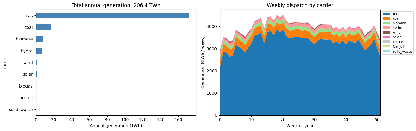
10.1 Annual generation by carrier

Total energy delivered by each carrier across all 472 buses and all 8760 hours, plus the same broken down by month to expose seasonality (hydro / solar peaks, dry-season thermal ramps).

annual = (
    gen_df.groupby('carrier')['value'].sum().sort_values(ascending=True) / 1e6
)  # MWh -> TWh
gen_df['week'] = ((gen_df['hour'] - 1) // (24 * 7)).clip(upper=51)
weekly = (
    gen_df.groupby(['week', 'carrier'])['value'].sum().unstack().fillna(0)
    / 1e3  # MWh -> GWh per week
)
fig, axes = plt.subplots(1, 2, figsize=(14, 4.5))
annual.plot.barh(ax=axes[0], color='steelblue')
axes[0].set_xlabel('Annual generation (TWh)')
axes[0].set_title(f'Total annual generation: {annual.sum():.1f} TWh')
weekly[annual.sort_values(ascending=False).index].plot.area(
    ax=axes[1], colormap='tab20', linewidth=0,
)
axes[1].set_xlabel('Week of year')
axes[1].set_ylabel('Generation (GWh / week)')
axes[1].set_title('Weekly dispatch by carrier')
axes[1].legend(loc='upper left', bbox_to_anchor=(1.0, 1.0), fontsize=8)
axes[1].set_xlim(0, 51)
plt.tight_layout(); plt.show()

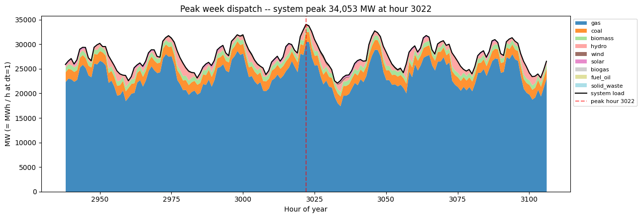
10.2 Peak-week hourly dispatch

Locate the hour with system-wide peak demand and stack the generation mix across the seven days surrounding it. This is the canonical “stress test” view of a PCM run: which carriers fill in on the highest-load day, and what the ramping pattern looks like.

sys_load = long_load.groupby('hour')['value'].sum().sort_index()
peak_h = int(sys_load.idxmax())
window_lo = max(1, peak_h - 84)
window_hi = min(8760, peak_h + 84)  # +/- 3.5 days

slice_gen = gen_df[(gen_df.hour >= window_lo) & (gen_df.hour <= window_hi)]
hourly_carrier = (
    slice_gen.groupby(['hour', 'carrier'])['value'].sum().unstack().fillna(0)
)
order = (
    gen_df.groupby('carrier')['value'].sum().sort_values(ascending=False).index
)
hourly_carrier = hourly_carrier[[c for c in order if c in hourly_carrier.columns]]

fig, ax = plt.subplots(figsize=(13, 4.5))
hourly_carrier.plot.area(ax=ax, colormap='tab20', linewidth=0, alpha=0.85)
ax.plot(sys_load.loc[window_lo:window_hi].index,
        sys_load.loc[window_lo:window_hi].values,
        color='black', linewidth=1.5, label='system load')
ax.axvline(peak_h, color='red', linestyle='--', alpha=0.6,
           label=f'peak hour {peak_h}')
ax.set_xlabel('Hour of year')
ax.set_ylabel('MW (= MWh / h at dt=1)')
ax.set_title(f'Peak week dispatch -- system peak {sys_load.max():,.0f} MW '
             f'at hour {peak_h}')
ax.legend(loc='upper left', bbox_to_anchor=(1.0, 1.0), fontsize=8)
plt.tight_layout(); plt.show()

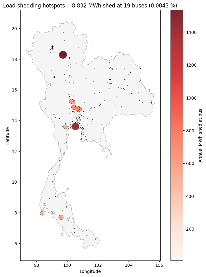
10.3 Load-shedding hotspots

Where on the network does the LP fall back to the VOLL slack? Each marker is sized by total annual MWh shed at that bus. With the current cap_source and full transmission topology this is typically tiny (hundreds to thousands of MWh on a 200 + TWh demand) – mostly small load pockets behind constrained 115 kV sub-networks.

lns_total = lns_df.groupby('zone')['value'].sum()
lns_pos = lns_total[lns_total > 0.001]

fig, ax = plt.subplots(figsize=(7, 9))
draw_thailand(ax)
ax.scatter(peak['lon'], peak['lat'], s=2, color='black', alpha=0.3,
           label=f'all buses ({len(peak)})')
if len(lns_pos):
    pts = pd.DataFrame({'zone': lns_pos.index, 'lns_mwh': lns_pos.values})
    pts['lon'] = pts['zone'].map(lambda z: bus_lonlat.get(z, (np.nan, np.nan))[0])
    pts['lat'] = pts['zone'].map(lambda z: bus_lonlat.get(z, (np.nan, np.nan))[1])
    pts = pts.dropna(subset=['lon', 'lat'])
    sc = ax.scatter(
        pts['lon'], pts['lat'],
        s=np.clip(pts['lns_mwh'] / 5, 8, 300),
        c=pts['lns_mwh'], cmap='Reds', alpha=0.85, zorder=3,
        edgecolor='black', linewidth=0.4,
    )
    fig.colorbar(sc, ax=ax, label='Annual MWh shed at bus')
    ax.set_title(
        f'Load-shedding hotspots -- {lns_pos.sum():,.0f} MWh shed '
        f'at {len(lns_pos)} buses ({100*lns_pos.sum()/long_load.value.sum():.4f} %)'
    )
else:
    ax.set_title('No load shedding (LP feasible at all hours)')
ax.set_xlabel('Longitude'); ax.set_ylabel('Latitude')
plt.tight_layout(); plt.show()

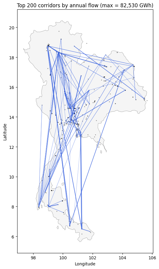
10.4 Top transmission corridors

Aggregate trans_export over the year to see which directed lines carry the most energy. Width on the map is proportional to total annual flow; the top-20 lines also get a tabular view.

line_total = trans_df.groupby(['zone1', 'zone2'])['value'].sum() / 1e3  # GWh
line_total = line_total.sort_values(ascending=False)
print('Top 10 directed lines by annual flow (GWh):')
print(line_total.head(10).to_string())

fig, ax = plt.subplots(figsize=(7, 9))
draw_thailand(ax)
ax.scatter(peak['lon'], peak['lat'], s=1.5, color='black', alpha=0.3)
top_n = 200  # plot top 200 corridors so the map isn't cluttered
top_lines = line_total.head(top_n)
norm = top_lines.max() if len(top_lines) else 1.0
for (z1, z2), gwh in top_lines.items():
    if z1 not in bus_lonlat or z2 not in bus_lonlat:
        continue
    sx, sy = bus_lonlat[z1]
    kx, ky = bus_lonlat[z2]
    ax.plot([sx, kx], [sy, ky],
            color='royalblue',
            linewidth=np.clip(3 * gwh / norm, 0.2, 3.0),
            alpha=0.6)
ax.set_xlabel('Longitude'); ax.set_ylabel('Latitude')
ax.set_title(f'Top {top_n} corridors by annual flow '
             f'(max = {top_lines.iloc[0]:,.0f} GWh)')
plt.tight_layout(); plt.show()

Top 10 directed lines by annual flow (GWh):
zone1   zone2
bus248  bus250    82529.520860
bus250  bus248    75625.947765
bus160  bus161    62416.880038
bus161  bus160    61305.151738
bus328  bus327    53902.603615
bus327  bus328    51080.280662
bus87   bus86     48476.762855
bus167  bus168    48330.486667
bus102  bus87     46135.550133
bus86   bus87     44965.737397

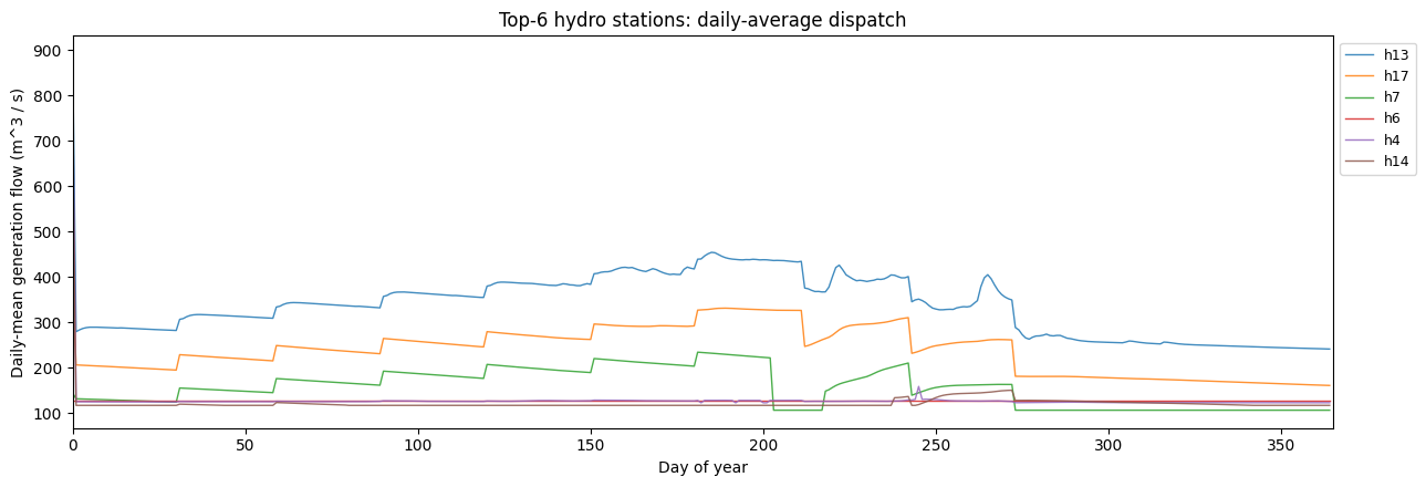
10.5 Hydro: per-station discharge profiles

Each cascading hydro station has its own water budget; this plot shows the daily-average generation flow for a few representative stations. Spillage stays at zero in this dataset (no binding storage_max), so we only show generation flow.

stations_by_total = (
    genflow_df.groupby('station')['value'].sum().sort_values(ascending=False)
)
print('Top 5 hydro stations by annual genflow (m^3 / s * h):')
print(stations_by_total.head(5).to_string())

# Daily mean per station for plotting -- 24h average smooths out
# diurnal noise and keeps 365 points per station.
genflow_df['day'] = ((genflow_df['hour'] - 1) // 24)
daily = (
    genflow_df.groupby(['day', 'station'])['value'].mean().unstack()
)

# Plot the top-6 stations.
top6 = stations_by_total.head(6).index
fig, ax = plt.subplots(figsize=(13, 4.5))
for s in top6:
    if s in daily.columns:
        ax.plot(daily.index, daily[s], linewidth=1.0, alpha=0.85, label=s)
ax.set_xlabel('Day of year')
ax.set_ylabel('Daily-mean generation flow (m^3 / s)')
ax.set_title('Top-6 hydro stations: daily-average dispatch')
ax.legend(loc='upper left', bbox_to_anchor=(1.0, 1.0), fontsize=9)
ax.set_xlim(0, 365)
plt.tight_layout(); plt.show()

Top 5 hydro stations by annual genflow (m^3 / s * h):
station
h13    2.966599e+06
h17    2.097796e+06
h7     1.372608e+06
h6     1.125588e+06
h4     1.119077e+06

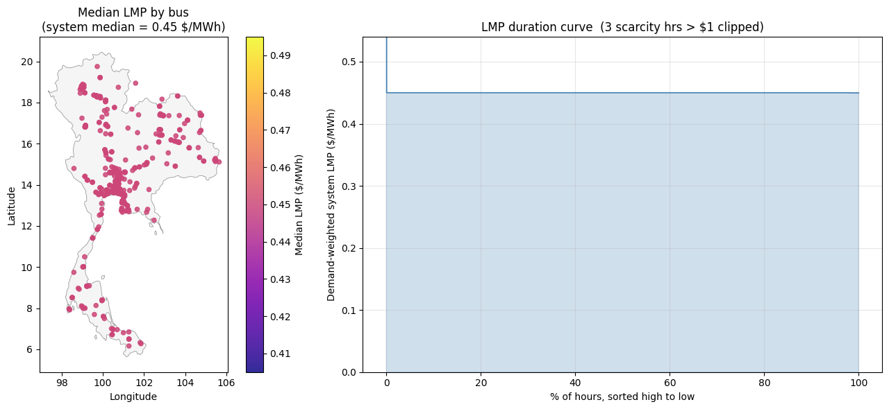
10.6 Locational marginal prices (LMP)

The shadow price of every nodal power-balance constraint, scaled back to real-year USD/MWh (raw dual times weight / var_factor), sign-flipped so positive means “more expensive to serve one more MWh at this bus”.

• Left: median LMP per bus on the map. The median is robust to the rare VOLL-saturated shortage hours, so the colour scale tracks the typical merit-order price at each bus.

• Right: demand-weighted system LMP, sorted high to low. The y-axis is clipped above the 99.9th percentile so the curve shape is readable; any scarcity hours that exceed the cap are noted in the title.

lmp_df = pd.read_parquet(PCM_OUT / 'lmp.parquet')

# Annual MEDIAN LMP per zone (median is robust to the rare VOLL
# spikes during shortage hours, so the colour scale tracks
# typical merit-order pricing at each bus rather than the
# shedding-frequency outliers).
mean_lmp = (
    lmp_df.groupby('zone')['value'].median()
    .rename('lmp_median').reset_index()
)
mean_lmp['lon'] = mean_lmp['zone'].map(lambda z: bus_lonlat.get(z, (np.nan, np.nan))[0])
mean_lmp['lat'] = mean_lmp['zone'].map(lambda z: bus_lonlat.get(z, (np.nan, np.nan))[1])
mean_lmp = mean_lmp.dropna(subset=['lon', 'lat'])

# System-wide LMP per hour: demand-weighted average across buses
# (so the duration view tracks what the average MWh paid).
demand_hr = (
    long_load[['hour', 'zone', 'value']]
    .rename(columns={'value': 'mw'})
)
joined = lmp_df.merge(demand_hr, on=['hour', 'zone'])
joined['weighted'] = joined['value'] * joined['mw']
sys_lmp = (
    joined.groupby('hour')[['weighted', 'mw']].sum()
    .assign(lmp=lambda d: d['weighted'] / d['mw'])['lmp']
    .sort_values(ascending=False).reset_index(drop=True)
)
# Headroom for the y-axis: a touch above the 99.9th percentile so
# the curve shape is visible without the rare scarcity spikes
# dictating the scale.
y_top = float(sys_lmp.quantile(0.999) * 1.2)
n_clipped = int((sys_lmp > y_top).sum())

fig, axes = plt.subplots(1, 2, figsize=(14, 6),
                         gridspec_kw={'width_ratios': [1, 1.4]})
draw_thailand(axes[0])
sc = axes[0].scatter(
    mean_lmp['lon'], mean_lmp['lat'],
    c=mean_lmp['lmp_median'], cmap='plasma',
    s=20, alpha=0.85,
    vmin=mean_lmp['lmp_median'].quantile(0.05),
    vmax=mean_lmp['lmp_median'].quantile(0.95),
)
axes[0].set_xlabel('Longitude'); axes[0].set_ylabel('Latitude')
axes[0].set_title(f'Median LMP by bus\n'
                  f'(system median = {mean_lmp["lmp_median"].median():.2f} $/MWh)')
fig.colorbar(sc, ax=axes[0], label='Median LMP ($/MWh)')

axes[1].plot(np.arange(len(sys_lmp)) / len(sys_lmp) * 100, sys_lmp.values,
             color='steelblue', linewidth=1.2)
axes[1].fill_between(np.arange(len(sys_lmp)) / len(sys_lmp) * 100,
                     0, sys_lmp.values, alpha=0.25, color='steelblue')
axes[1].set_ylim(0, y_top)
axes[1].set_xlabel('% of hours, sorted high to low')
axes[1].set_ylabel('Demand-weighted system LMP ($/MWh)')
title = 'LMP duration curve'
if n_clipped:
    title += f'  ({n_clipped} scarcity hrs > ${y_top:.0f} clipped)'
axes[1].set_title(title)
axes[1].grid(True, alpha=0.3)
plt.tight_layout(); plt.show()