Run online (zero install): Open in Binder or Open in Colab. Binder is anonymous; Colab needs a Google account but starts faster.
Run locally: clone the repo and install with the notebook extra:
git clone https://github.com/PREP-NexT/PREP-SHOT.git
cd PREP-SHOT
pip install -e .[notebook]
jupyter lab doc/source/Quickstart.ipynb
[ ]:
# On Google Colab, install PREP-SHOT and clone the repo so the
# path-walk below can locate run.py / config.json. No-op on
# Binder / local where prepshot is already importable.
try:
    import google.colab  # type: ignore  # noqa: F401
    IS_COLAB = True
except ImportError:
    IS_COLAB = False

if IS_COLAB:
    import os
    if not os.path.isdir('/content/PREP-SHOT'):
        !git clone --depth=1 https://github.com/PREP-NexT/PREP-SHOT.git /content/PREP-SHOT
    %cd /content/PREP-SHOT
    !pip install --quiet -e .
    !pip install --quiet matplotlib h5netcdf
Quickstart (30 minutes)
Goal: take a fresh checkout of PREP-SHOT, solve the shipped example, read the results, change one input, and re-solve – all in about half an hour. No prior knowledge of capacity-expansion modeling is assumed; everything happens against the input/ folder that comes with the repo.
If anything in this page does not work for you, please open a GitHub issue – we read every report and a broken Quickstart is the bug we most want to know about.
Step 1 – Install (5 minutes)
PREP-SHOT requires Python 3.9 or newer. Conda is recommended so the optimization-solver dependencies stay isolated:
conda create -n prep-shot python=3.11 -y
conda activate prep-shot

git clone https://github.com/PREP-NexT/PREP-SHOT.git
cd PREP-SHOT
pip install -e .
The default solver is the open-source HiGHS, installed automatically as a wheel. To use a commercial solver (Gurobi, COPT, MOSEK) instead, set solver in config.json – see the Model Inputs/Outputs page.
Step 2 – Solve the shipped example (5 minutes)
The repo ships a self-contained 3-zone, 11-year example in input/. We solve it programmatically so this notebook works regardless of the working directory.
[1]:
import sys
import io
import pathlib

# Notebooks inherit the kernel launcher's argv; clear it so
# prepshot.set_up.parse_cli_arguments() sees no scenario flags.
sys.argv = ['notebook']

# Locate the repo root (the dir containing run.py and config.json).
# This makes the notebook portable: it works from doc/source/, from
# the repo root, or from any subdirectory of a checkout.
repo_root = pathlib.Path.cwd()
while not (repo_root / 'run.py').exists():
    if repo_root == repo_root.parent:
        raise RuntimeError(
            'Could not find PREP-SHOT repo root; run this notebook '
            'from inside a checkout of PREP-NexT/PREP-SHOT.'
        )
    repo_root = repo_root.parent
print(f'PREP-SHOT repo root: {repo_root}')
PREP-SHOT repo root: /Users/energy/01-doing/PREP-SHOT-tutorial/PREP-SHOT
[2]:
import os
import sys
import tempfile
from prepshot.cli import main

# HiGHS writes its progress log via C-level stdout (file
# descriptor 1), which bypasses Python's sys.stdout. Redirect
# the file descriptor to a tempfile during the solve so the
# notebook output stays readable; we keep a path to the log so
# the next cell can extract the final objective.
with tempfile.NamedTemporaryFile('w+', delete=False, prefix='prepshot_solve_') as f:
    log_path = f.name
    sys.stdout.flush()
    saved_fd = os.dup(1)
    os.dup2(f.fileno(), 1)
    try:
        solved = main(root_dir=str(repo_root))
    finally:
        sys.stdout.flush()
        os.dup2(saved_fd, 1)
        os.close(saved_fd)
print(f'log: {log_path}')
2026-05-03 19:18:30 INFO: Set parameter solver to value highs
2026-05-03 19:18:30 INFO: Set parameter input folder to value input
2026-05-03 19:18:30 INFO: Set parameter output_filename to value year.nc
2026-05-03 19:18:30 INFO: Set parameter time_length to value 48
2026-05-03 19:18:30 INFO: Start running 'create_model'
2026-05-03 19:18:30 INFO: Loaded HiGHS library: /Users/energy/miniconda3/envs/prep-shot/lib/python3.9/site-packages/highsbox/highs_dist/lib/libhighs.dylib
2026-05-03 19:18:30 INFO: Loaded highs library automatically.
2026-05-03 19:18:32 INFO: Finished 'create_model' in 1.12 seds
2026-05-03 19:18:32 INFO: Start running 'solve_model'
2026-05-03 19:18:32 INFO: Starting iteration recorded at 2026-05-03 19:18:32.
2026-05-03 19:18:45 INFO: Water head error: 564.63%
2026-05-03 19:19:42 INFO: Water head error: 8.91%
2026-05-03 19:20:20 INFO: Water head error: 9.46%
2026-05-03 19:20:20 WARNING: Ending iteration recorded at 2026-05-03 19:20:20.Failed to converge. Maximum iteration exceeded.
2026-05-03 19:20:20 INFO: Finished 'solve_model' in 108.78 seds
2026-05-03 19:20:20 INFO: Start running 'extract_results_hydro'
2026-05-03 19:20:20 INFO: Start running 'extract_results_non_hydro'
2026-05-03 19:20:20 INFO: Finished 'extract_results_non_hydro' in 0.03 seds
2026-05-03 19:20:20 INFO: Finished 'extract_results_hydro' in 0.03 seds
2026-05-03 19:20:21 INFO: Results are written to ./output/year.nc
2026-05-03 19:20:21 INFO: Start running 'save_to_excel'
2026-05-03 19:20:25 INFO: Finished 'save_to_excel' in 4.43 seds
2026-05-03 19:20:25 INFO: Results are written to separate excel files
log: /var/folders/y_/ypyrt83d1hl9fhjtt_ftpwg00000gn/T/prepshot_solve_1j_icnsv
[3]:
# Pick out the final objective value from the captured log.
with open(log_path) as f:
    log = f.read()
objective_lines = [l for l in log.splitlines() if 'Objective value' in l]
if objective_lines:
    # The solve runs `iteration_number` head iterations; each
    # prints an objective. The last one is what matters.
    print(objective_lines[-1].strip())
print(f'Solved: {solved}')
Objective value     :  1.8805577710e+11
Solved: True
On commodity hardware the default settings (48 hours, 1 representative month, 3 head iterations) finish in around 2 minutes. The solver log will report Objective value : 1.8809...e+11, and a NetCDF file appears under output/. Everything in the rest of this notebook reads from that file.
The log lines Water head error: ... and the warning Failed to converge. Maximum iteration exceeded. are normal for the default settings: PREP-SHOT runs three head-iteration rounds and reports the final residual. Bump iteration_number in config.json if you want a tighter (slower) converged solve.
Step 3 – Open the results (10 minutes)
PREP-SHOT writes results in xarray’s NetCDF format, so any tool that reads NetCDF can consume them.
[4]:
import xarray as xr
import json

config = json.loads((repo_root / 'config.json').read_text())
# config stores the filename WITHOUT extension; the model writes
# both .nc (xarray) and .xlsx alongside each other.
output_path = (
    repo_root
    / 'output'
    / (config['general_parameters']['output_filename'] + '.nc')
)
print(f'Reading results from: {output_path}')

ds = xr.open_dataset(output_path)
print(sorted(ds.data_vars))
Reading results from: /Users/energy/01-doing/PREP-SHOT-tutorial/PREP-SHOT/output/year.nc
['carbon', 'carbon_breakdown', 'charge', 'cost', 'cost_fix', 'cost_fix_breakdown', 'cost_newline', 'cost_newline_breakdown', 'cost_newtech', 'cost_newtech_breakdown', 'cost_var', 'cost_var_breakdown', 'gen', 'genflow', 'income', 'install', 'public_debt_newtech', 'shadow_price_demand', 'spillflow', 'trans_export']
Three things worth a first look:
1. Total cost. A single number, the NPV of system cost over the planning horizon.
[5]:
print(f"Total cost: ${float(ds.cost):,.0f}")
Total cost: $188,055,777,096
2. Installed capacity over time. Which technologies expanded, in which zones, and when.
[6]:
install_by_year = ds["install"].sum("zone").to_pandas()
install_by_year
[6]:
| tech | Coal | Solar | Wind | Storage | Grand_Coulee | Chief_Joseph | Wells | Rocky_Reach | Rock_Island | Wanapum | Priest_Rapids | Lower_Granite | Little_Goose | Lower_Monumental | Ice_Harbor | McNary | John_Day | The_Dalles | Bonneville |
|---|---|---|---|---|---|---|---|---|---|---|---|---|---|---|---|---|---|---|---|
| year | |||||||||||||||||||
| 2020 | 34.526238 | 0.000000 | 28045.085013 | 0.0 | 5054.0 | 2234.0 | 741.0 | 1126.0 | 482.0 | 890.0 | 828.0 | 747.0 | 748.0 | 784.0 | 525.0 | 1022.0 | 1943.0 | 1414.0 | 921.0 |
| 2021 | 34.526238 | 0.000000 | 28045.085013 | 0.0 | 5054.0 | 2234.0 | 741.0 | 1126.0 | 482.0 | 890.0 | 828.0 | 747.0 | 748.0 | 784.0 | 525.0 | 1022.0 | 1943.0 | 1414.0 | 921.0 |
| 2022 | 34.526238 | 0.000000 | 28045.085013 | 0.0 | 5054.0 | 2234.0 | 741.0 | 1126.0 | 482.0 | 890.0 | 828.0 | 747.0 | 748.0 | 784.0 | 525.0 | 1022.0 | 1943.0 | 1414.0 | 921.0 |
| 2023 | 34.526238 | 0.000000 | 28045.085013 | 0.0 | 5054.0 | 2234.0 | 741.0 | 1126.0 | 482.0 | 890.0 | 828.0 | 747.0 | 748.0 | 784.0 | 525.0 | 1022.0 | 1943.0 | 1414.0 | 921.0 |
| 2024 | 34.526238 | 19246.734302 | 28045.085013 | 0.0 | 5054.0 | 2234.0 | 741.0 | 1126.0 | 482.0 | 890.0 | 828.0 | 747.0 | 748.0 | 784.0 | 525.0 | 1022.0 | 1943.0 | 1414.0 | 921.0 |
| 2025 | 34.526238 | 19246.734302 | 28045.085013 | 0.0 | 5054.0 | 2234.0 | 741.0 | 1126.0 | 482.0 | 890.0 | 828.0 | 747.0 | 748.0 | 784.0 | 525.0 | 1022.0 | 1943.0 | 1414.0 | 921.0 |
| 2026 | 34.526238 | 26519.619727 | 29965.811926 | 0.0 | 5054.0 | 2234.0 | 741.0 | 1126.0 | 482.0 | 890.0 | 828.0 | 747.0 | 748.0 | 784.0 | 525.0 | 1022.0 | 1943.0 | 1414.0 | 921.0 |
| 2027 | 34.526238 | 26519.619727 | 29965.811926 | 0.0 | 5054.0 | 2234.0 | 741.0 | 1126.0 | 482.0 | 890.0 | 828.0 | 747.0 | 748.0 | 784.0 | 525.0 | 1022.0 | 1943.0 | 1414.0 | 921.0 |
| 2028 | 34.526238 | 26519.619727 | 29965.811926 | 0.0 | 5054.0 | 2234.0 | 741.0 | 1126.0 | 482.0 | 890.0 | 828.0 | 747.0 | 748.0 | 784.0 | 525.0 | 1022.0 | 1943.0 | 1414.0 | 921.0 |
| 2029 | 34.526238 | 39296.605613 | 29965.811926 | 0.0 | 5054.0 | 2234.0 | 741.0 | 1126.0 | 482.0 | 890.0 | 828.0 | 747.0 | 748.0 | 784.0 | 525.0 | 1022.0 | 1943.0 | 1414.0 | 921.0 |
| 2030 | 34.526238 | 39296.605613 | 29965.811926 | 0.0 | 5054.0 | 2234.0 | 741.0 | 1126.0 | 482.0 | 890.0 | 828.0 | 747.0 | 748.0 | 784.0 | 525.0 | 1022.0 | 1943.0 | 1414.0 | 921.0 |
3. Locational marginal prices (shadow prices on demand). This is the dual of the power-balance constraint – the marginal cost of one extra MWh of demand at each (hour, month, year, zone). Useful for diagnosing where the system is most stressed.
[7]:
# LMP at zone BA1 in 2025, averaged over the modeled month:
lmp = ds["shadow_price_demand"].sel(zone="BA1", year=2025).mean("month")
print(lmp)
<xarray.DataArray 'shadow_price_demand' (hour: 48)> Size: 384B
array([0.00000000e+00, 0.00000000e+00, 1.68494800e-13, 0.00000000e+00,
       0.00000000e+00, 0.00000000e+00, 0.00000000e+00, 0.00000000e+00,
       0.00000000e+00, 0.00000000e+00, 0.00000000e+00, 0.00000000e+00,
       0.00000000e+00, 0.00000000e+00, 0.00000000e+00, 0.00000000e+00,
       0.00000000e+00, 7.81236838e-03, 0.00000000e+00, 0.00000000e+00,
       0.00000000e+00, 0.00000000e+00, 0.00000000e+00, 0.00000000e+00,
       0.00000000e+00, 0.00000000e+00, 0.00000000e+00, 0.00000000e+00,
       0.00000000e+00, 0.00000000e+00, 0.00000000e+00, 0.00000000e+00,
       0.00000000e+00, 0.00000000e+00, 0.00000000e+00, 0.00000000e+00,
       0.00000000e+00, 0.00000000e+00, 0.00000000e+00, 0.00000000e+00,
       0.00000000e+00, 8.08277773e-13, 0.00000000e+00, 0.00000000e+00,
       0.00000000e+00, 0.00000000e+00, 0.00000000e+00, 0.00000000e+00])
Coordinates:
  * hour     (hour) int64 384B 1 2 3 4 5 6 7 8 9 ... 40 41 42 43 44 45 46 47 48
    year     int64 8B 2025
    zone     <U3 12B 'BA1'
Values in shadow_price_demand are NPV-discounted dollars per MWh. To recover undiscounted real-year prices, divide by the year’s variable-cost factor (computed in prepshot.load_data.compute_cost_factors).
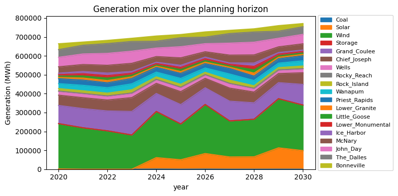
A minimal generation-mix chart:
[8]:
%matplotlib inline
import matplotlib.pyplot as plt

gen_by_tech = (
    ds["gen"]
    .sum(["hour", "month", "zone"])  # sum over time and space
    .to_pandas()                     # rows=year, cols=tech
    .clip(lower=0)                   # storage net-discharge can be ~0; clamp
)
# Drop techs that never generate (e.g. storage round-trips to ~0):
gen_by_tech = gen_by_tech.loc[:, gen_by_tech.sum() > 0]

fig, ax = plt.subplots(figsize=(8, 4))
gen_by_tech.plot.area(ax=ax)
ax.set_ylabel("Generation (MWh)")
ax.set_title("Generation mix over the planning horizon")
ax.legend(loc="center left", bbox_to_anchor=(1.0, 0.5), fontsize=8)
fig.tight_layout()
plt.show()
Step 4 – Change one input and re-solve (5 minutes)
Every input is a CSV under input/. To see how the model responds to a change, try one of these single-file edits.
Option A – bump demand 20% in one zone. Open input/demand.csv (long format: zone, year, month, hour, unit, value) and multiply the BA1 column by 1.2 in your editor of choice. Then run python run.py again. The objective will rise – the model has to build more capacity or import more from neighboring zones to serve the extra load. shadow_price_demand at BA1 should also increase in the most constrained hours.
Option B – introduce a carbon tax. Open input/policy_carbon_tax.csv and replace the value column with a non-zero number (e.g. 50 USD/tonneCO2). Re-run; the generation mix should shift away from coal and gas toward zero-carbon technologies, raising cost_carbon in the breakdown.
Tip – run scenarios without overwriting your baseline. Save your modified file as input/demand_high.csv and run python run.py --demand=high. PREP-SHOT appends the suffix to the file name, so the baseline demand.csv is left untouched. Output goes to output/year_high.nc.
Step 5 – Where to next
Model Inputs/Outputs – full input / output reference, including optional carbon-market and finance modules.
Tutorial – the same shipped example, with more context on the modeled scenario (3 balancing authorities, 15 hydropower stations, 2020-2030 zero-carbon pathway).
Mathematical Notation – the underlying linear program.
Changelog – what’s new in each release.
If you used PREP-SHOT in published work, please cite it – see the Citation Guide. And if you ran into something rough, the fastest fix is to file an issue on GitHub.